
The GNMT v2 model is an improved version of the first Google's Neural Machine Translation System with a modified attention mechanism.
This resource is using open-source code maintained in github (see the quick-start-guide section) and available for download from NGC
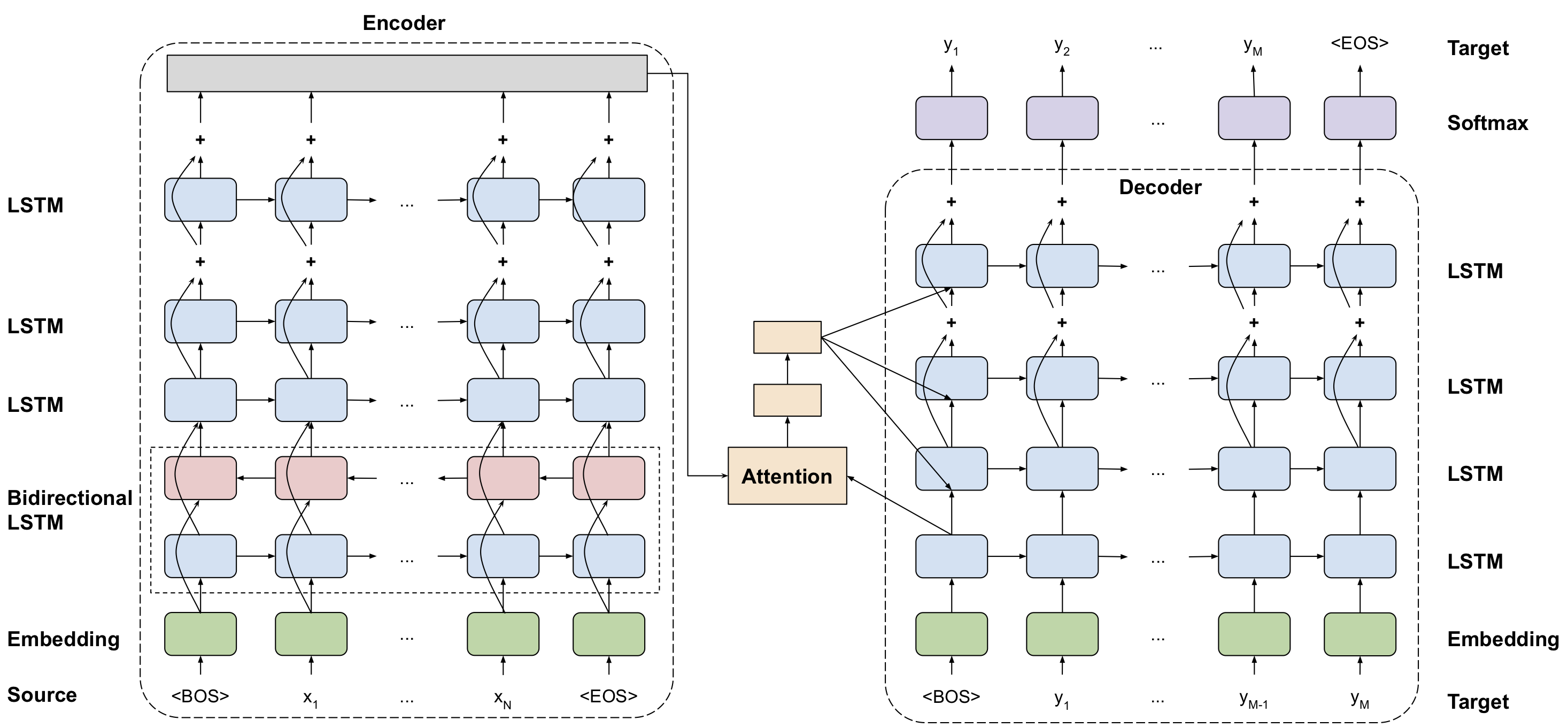
The GNMT v2 model is similar to the one discussed in the Google's Neural Machine Translation System: Bridging the Gap between Human and Machine Translation paper.
The most important difference between the two models is in the attention mechanism. In our model, the output from the first LSTM layer of the decoder goes into the attention module, then the re-weighted context is concatenated with inputs to all subsequent LSTM layers in the decoder at the current time step.
The same attention mechanism is also implemented in the default GNMT-like models from TensorFlow Neural Machine Translation Tutorial and NVIDIA OpenSeq2Seq Toolkit.
Model architecture
Default configuration
The following features were implemented in this model:
- general:
- encoder and decoder are using shared embeddings
- data-parallel multi-GPU training
- dynamic loss scaling with backoff for Tensor Cores (mixed precision) training
- trained with label smoothing loss (smoothing factor 0.1)
- encoder:
- 4-layer LSTM, hidden size 1024, first layer is bidirectional, the rest are unidirectional
- with residual connections starting from 3rd layer
- uses standard PyTorch nn.LSTM layer
- dropout is applied on input to all LSTM layers, probability of dropout is set to 0.2
- hidden state of LSTM layers is initialized with zeros
- weights and bias of LSTM layers is initialized with uniform(-0.1,0.1) distribution
- decoder:
- 4-layer unidirectional LSTM with hidden size 1024 and fully-connected classifier
- with residual connections starting from 3rd layer
- uses standard PyTorch nn.LSTM layer
- dropout is applied on input to all LSTM layers, probability of dropout is set to 0.2
- hidden state of LSTM layers is initialized with zeros
- weights and bias of LSTM layers is initialized with uniform(-0.1,0.1) distribution
- weights and bias of fully-connected classifier is initialized with uniform(-0.1,0.1) distribution
- attention:
- normalized Bahdanau attention
- output from first LSTM layer of decoder goes into attention, then re-weighted context is concatenated with the input to all subsequent LSTM layers of the decoder at the current timestep
- linear transform of keys and queries is initialized with uniform(-0.1, 0.1), normalization scalar is initialized with 1.0/sqrt(1024), normalization bias is initialized with zero
- inference:
- beam search with default beam size of 5
- with coverage penalty and length normalization, coverage penalty factor is set to 0.1, length normalization factor is set to 0.6 and length normalization constant is set to 5.0
- de-tokenized BLEU computed by SacreBLEU
- motivation for choosing SacreBLEU
When comparing the BLEU score, there are various tokenization approaches and BLEU calculation methodologies; therefore, ensure you align similar metrics.
Code from this repository can be used to train a larger, 8-layer GNMT v2 model.
Our experiments show that a 4-layer model is significantly faster to train and
yields comparable accuracy on the public WMT16
English-German dataset. The
number of LSTM layers is controlled by the --num-layers parameter in the
train.py training script.
Feature support matrix
The following features are supported by this model.
| Feature | GNMT v2 |
|---|---|
| Apex AMP | Yes |
| Apex DistributedDataParallel | Yes |
Features
Apex AMP - a tool that enables Tensor Core-accelerated training. Refer to the Enabling mixed precision section for more details.
Apex
DistributedDataParallel -
a module wrapper that enables easy multiprocess distributed data parallel
training, similar to
torch.nn.parallel.DistributedDataParallel.
DistributedDataParallel is optimized for use with
NCCL. It achieves high performance by
overlapping communication with computation during backward() and bucketing
smaller gradient transfers to reduce the total number of transfers required.
Mixed precision training
Mixed precision is the combined use of different numerical precisions in a computational method. Mixed precision training offers significant computational speedup by performing operations in half-precision format, while storing minimal information in single-precision to retain as much information as possible in critical parts of the network. Since the introduction of Tensor Cores in Volta, and following with both the Turing and Ampere architectures, significant training speedups are experienced by switching to mixed precision -- up to 3x overall speedup on the most arithmetically intense model architectures. Using mixed precision training previously required two steps:
- Porting the model to use the FP16 data type where appropriate.
- Manually adding loss scaling to preserve small gradient values.
The ability to train deep learning networks with lower precision was introduced in the Pascal architecture and first supported in CUDA 8 in the NVIDIA Deep Learning SDK.
For information about:
- How to train using mixed precision, see the Mixed Precision Training paper and Training With Mixed Precision documentation.
- Techniques used for mixed precision training, see the Mixed-Precision Training of Deep Neural Networks blog.
- APEX tools for mixed precision training, see the NVIDIA Apex: Tools for Easy Mixed-Precision Training in PyTorch .
Enabling mixed precision
Mixed precision is enabled in PyTorch by using the Automatic Mixed Precision
(AMP), library from APEX that casts variables
to half-precision upon retrieval, while storing variables in single-precision
format. Furthermore, to preserve small gradient magnitudes in backpropagation,
a loss
scaling
step must be included when applying gradients. In PyTorch, loss scaling can be
easily applied by using scale_loss() method provided by AMP. The scaling
value to be used can be
dynamic or fixed.
For an in-depth walk through on AMP, check out sample usage here. APEX is a PyTorch extension that contains utility libraries, such as AMP, which require minimal network code changes to leverage Tensor Cores performance.
The following steps were needed to enable mixed precision training in GNMT:
- Import AMP from APEX (file:
seq2seq/train/trainer.py):
from apex import amp
- Initialize AMP and wrap the model and the optimizer (file:
seq2seq/train/trainer.py, class:Seq2SeqTrainer):
self.model, self.optimizer = amp.initialize(
    self.model,
    self.optimizer,
    cast_model_outputs=torch.float16,
    keep_batchnorm_fp32=False,
    opt_level='O2')
- Apply
scale_losscontext manager (file:seq2seq/train/fp_optimizers.py, class:AMPOptimizer):
with amp.scale_loss(loss, optimizer) as scaled_loss:
    scaled_loss.backward()
- Apply gradient clipping on single precision master weights (file:
seq2seq/train/fp_optimizers.py, class:AMPOptimizer):
if self.grad_clip != float('inf'):
    clip_grad_norm_(amp.master_params(optimizer), self.grad_clip)
Enabling TF32
TensorFloat-32 (TF32) is the new math mode in NVIDIA A100 GPUs for handling the matrix math also called tensor operations. TF32 running on Tensor Cores in A100 GPUs can provide up to 10x speedups compared to single-precision floating-point math (FP32) on Volta GPUs.
TF32 Tensor Cores can speed up networks using FP32, typically with no loss of accuracy. It is more robust than FP16 for models which require high dynamic range for weights or activations.
For more information, refer to the TensorFloat-32 in the A100 GPU Accelerates AI Training, HPC up to 20x blog post.
TF32 is supported in the NVIDIA Ampere GPU architecture and is enabled by default.